Polarization

Note

This section covers functionality that is still under development.

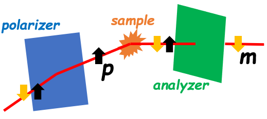
Polarized neutron beam experiments employ either half polarization, where the incident beam is polarized and the scattered beam is not analyzed, or full polarization, where the incident beam is polarized and the polarization of the scattered beam is also analyzed. The use of half or full polarization in a SANS experiment requires parsing the data into states corresponding to the states of the flipper, and the analyzer that is located between the sample and the detector.

Beam polarization and polarization ratio

The wavelength-dependent polarization of the incident beam that is defined by the polarizer is denoted \(P(\lambda)\). In the following, it is assumed that the polarizer produces the spin-up state, which would be true for a reflection polarizer. If a transmission polarizer, which produces the spin-down state, is employed, then the states derived from the measured flipper and analyzer conditions, described below, are reversed.

\(P(\lambda)\) is related to the instantaneous populations of spin-up and spin-down neutrons in the beam, denoted \(N^{\uparrow}(\lambda)\) and \(N^{\downarrow}(\lambda)\), respectively, through Equation (1).

(1)\[P(\lambda) = \frac{N^{\uparrow}(\lambda)-N^{\downarrow}(\lambda)}{N^{\uparrow}(\lambda)+N^{\downarrow}(\lambda)}\]

The wavelength-dependent polarization ratio \(R(\lambda)\), often called the flipping ratio, is defined by Equation (2).

(2)\[R(\lambda) = \frac{N^{\uparrow}(\lambda)}{N^{\downarrow}(\lambda)}\]

Then, \(R(\lambda)\) can be expressed in terms of \(P(\lambda)\) by Equation (3).

(3)\[R(\lambda) = \frac{1 + P(\lambda)}{1 - P(\lambda)}\]

Data splitting by polarizer and analyzer states

During data reduction, the event stream of data is parsed into workspaces representing the states of the polarizer and analyzer. Here, the notation used in the rest of this section is simplified by abbreviating any polarizer or analyzer state SANS data \(S(x,y,\lambda)\) as \(S(\lambda)\). When half polarization is employed, the “off” and “on” states of the flipper are measured , and the data are denoted \(S^0(\lambda)\) and \(S^1(\lambda)\), respectively. The quantities of interest in a half polarization measurement are the spin-up and spin-down state SANS data sets, denoted \(S^{\uparrow}(\lambda)\) and \(S^{\downarrow}(\lambda)\), respectively, which are related to the measured states.

Using full polarization introduces two additional conditions for when the analyzer is set to either \(0^{\circ}\) or \(180^{\circ}\). As a result, four SANS data sets are measured, which are denoted \(S^{00}(\lambda)\), \(S^{0\pi}(\lambda)\), \(S^{10}(\lambda)\) and \(S^{1\pi}(\lambda)\). By analogy with half polarization, there are four spin state SANS data sets of interest in a full polarization experiment, namely \(S^{\uparrow\uparrow}(\lambda)\), \(S^{\uparrow\downarrow}(\lambda)\), \(S^{\downarrow\uparrow}(\lambda)\) and \(S^{\downarrow\downarrow}(\lambda)\), that are related to the four measured polarization states.

Half polarization - polarized beam without polarization analysis

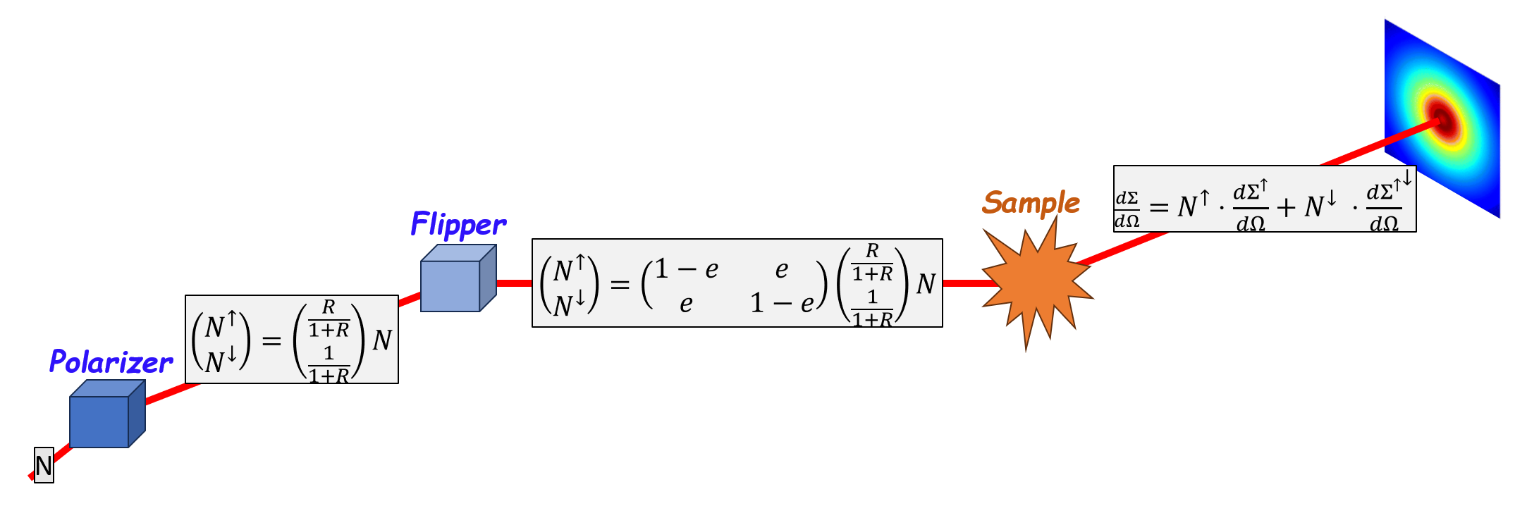
Half polarization experiments use a spin flipper with a wavelength-dependent efficiency \(e(\lambda)\) between the polarizer and the sample to rotate the spins from up to down, or vice versa depending on the polarizer in use. Consider the case that the flipper is off. The fractions of the beam that are spin-up and spin down, denoted \(f_{up}\) and \(f_{down}\), respectively, are given by Equations (4) and (5), respectively, and sample the spin-up scattering \(S^{\uparrow}(\lambda)\) and spin-down scattering \(S^{\downarrow}(\lambda)\).

(4)\[f_{up} = \frac{N^{\uparrow}}{N^{\uparrow}+N^{\downarrow}} = \frac{R(\lambda)}{1+R(\lambda)}\]

(5)\[f_{down} = \frac{N^{\downarrow}}{N^{\uparrow}+N^{\downarrow}} = \frac{1}{1+R(\lambda)}\]

Then, the total scattering measured by the detector for the off state is given by Equation (6), and its uncertainty is given by Equation (7).

(6)\[S^0(\lambda) = \frac{R(\lambda)}{1+R(\lambda)} S^{\uparrow}(\lambda) + \frac{1}{1+R(\lambda)} S^{\downarrow}(\lambda)\]

(7)\[(\delta S^0(\lambda))^2 = \left(\frac{R(\lambda)}{1+R(\lambda)}\right)^2 \left(\delta S^{\uparrow}(\lambda)\right)^2 + \left(\frac{1}{1+R(\lambda)}\right)^2 \left(\delta S^{\downarrow}(\lambda)\right)^2\]

When the flipper is on, it rotates the spins in the beam produced by the polarizer by \(\pi\) with an efficiency \(e(\lambda)\). The flipped spins are sensitive to the spin-down scattering state. The total scattering measured when the flipper is on, and its uncertainty are given by Equations (8) and (9), respectively.

(8)\[\begin{split}S^1(\lambda) = \left[ e(\lambda) \frac{1}{1+R(\lambda)} + (1-e(\lambda)) \frac{R(\lambda)}{1+R(\lambda)} \right] S^{\uparrow}(\lambda) + \\ \left[ e(\lambda) \frac{R(\lambda)}{1+R(\lambda)} + (1-e(\lambda)) \frac{1}{1+R(\lambda)} \right] S^{\downarrow}(\lambda)\end{split}\]

(9)\[\begin{split}(\delta S^1(\lambda))^2 = \left[ e(\lambda) \frac{1}{1+R(\lambda)} + (1-e(\lambda)) \frac{R(\lambda)}{1+R(\lambda)} \right]^2 \left(\delta S^{\uparrow}(\lambda)\right)^2 + \\ \left[ e(\lambda) \frac{R(\lambda)}{1+R(\lambda)} + (1-e(\lambda)) \frac{1}{1+R(\lambda)} \right]^2 \left(\delta S^{\downarrow}(\lambda)\right)^2\end{split}\]

As can be seen in Equations (6) through (9), the measurements produce data that contain mixtures of both states. The spin-up and spin-down SANS data, along with the associated uncertainties, are obtained by performing two \(2 \times 2\) matrix inversions. The matrices are the coefficients in Equations (6) and (8), which is denoted \(M_1\), and the coefficients in Equations (9) and (9), which is denoted \(M_2\). The matrix equations are shown in Equations (10) and (11) and are functions of wavelength. These equations no longer abbreviate the x and y dimensions of the SANS data.

(10)\[\begin{split}\begin{pmatrix} S^{\uparrow}(x, y, \lambda) \\ S^{\downarrow}(x, y, \lambda) \end{pmatrix} = M_1^{-1} \begin{pmatrix} S^0(x, y, \lambda) \\ S^1(x, y, \lambda) \end{pmatrix}\end{split}\]

(11)\[\begin{split}\begin{pmatrix} \delta S^{\uparrow}(x, y, \lambda)^2 \\ \delta S^{\downarrow}(x, y, \lambda)^2 \end{pmatrix} = M_1^{-1} \begin{pmatrix} \delta S^0(x, y, \lambda)^2 \\ \delta S^1(x, y, \lambda)^2 \end{pmatrix}\end{split}\]

Solving for \(S^{\uparrow}(x, y, \lambda)\), \(S^{\downarrow}(x, y, \lambda)\) yields the following equations.

(12)\[S^{\uparrow}(x, y, \lambda) = S^0(x, y, \lambda) + \frac{1}{e(\lambda)[R(\lambda)-1]} \left[ S^0(x, y, \lambda) - S^1(x, y, \lambda) \right]\]

(13)\[S^{\downarrow}(x, y, \lambda) = S^0(x, y, \lambda) + \frac{1}{e(\lambda)[1 - 1/R(\lambda)]} \left[ S^0(x, y, \lambda) - S^1(x, y, \lambda) \right]\]

Similarly, \(\delta S^{\uparrow}(x, y, \lambda)\) and \(\delta S^{\downarrow}(x, y, \lambda)\) can be solved for if we let the uncertainty in the efficiency of the polarizer be \(\delta e(\lambda)\) and \(\delta R(\lambda) \sim \left( 2/(1-P(\lambda))^2 \right) \delta P(\lambda)\), where \(\delta P(\lambda)\) is the uncertainty in the efficiency of the polarizer. The resulting expressions are shown in Equations (14) and (15).

(14)\[\begin{split}\left( \delta S^{\uparrow}(x, y, \lambda) \right)^2 = &\left(1+\frac{1}{e(\lambda)[R(\lambda)-1]}\right)^2 \left(\delta S^0(x,y,\lambda)\right)^2 + \\ &\left(\frac{1}{e(\lambda)[R(\lambda)-1]}\right)^2 \left(\delta S^1(x,y,\lambda)\right)^2 + \\ &\left(\frac{S^0(x,y,\lambda)-S^1(x,y,\lambda)}{e(\lambda)[R(\lambda)-1]}\right)^2 \left( \left(\frac{\delta e(\lambda)}{e(\lambda)}\right)^2 + \left(\frac{\delta R(\lambda)}{R(\lambda)-1}\right)^2 \right)\end{split}\]

(15)\[\begin{split}\left( \delta S^{\downarrow}(x, y, \lambda) \right)^2 = &\left(1+\frac{1}{e(\lambda)[1-1/R(\lambda)]}\right)^2 \left(\delta S^0(x,y,\lambda)\right)^2 + \\ &\left(\frac{1}{e(\lambda)[1-1/R(\lambda)]}\right)^2 \left(\delta S^1(x,y,\lambda)\right)^2 + \\ &\left(\frac{S^0(x,y,\lambda)-S^1(x,y,\lambda)}{e(\lambda)[1-1/R(\lambda)]} \right)^2 \left( \left(\frac{\delta e(\lambda)}{e(\lambda)}\right)^2 + \frac{1}{R(\lambda)^4} \left(\frac{\delta R(\lambda)}{1-1/R(\lambda)}\right)^2 \right)\end{split}\]

Full polarization - polarized beam with polarization analysis

When full polarization is employed, a \(^3\)He spin filter is inserted between the sample and the detector. The filter is also a spin flipper that rotates the spin by 0° or 180° and the polarizations of the two states of the \(^3\)He spin filter are denoted by \(A^0(\lambda)\) and \(A^{\pi}(\lambda)\). The 0° state is assumed to preferentially pass the spin-up state, but the software must allow for the reverse to be true. The four possible flipper states are related to the four spin states through Equations (16) through (19).

(16)\[\begin{split}S^{00}(\lambda) = \frac{R(\lambda)}{1+R(\lambda)} \frac{A^0(\lambda)}{1+A^0(\lambda)} S^{\uparrow\uparrow}(\lambda) + \frac{R(\lambda)}{1+R(\lambda)} \frac{1}{1+A^0(\lambda)} S^{\uparrow\downarrow}(\lambda) + \\ \frac{1}{1+R(\lambda)} \frac{A^0(\lambda)}{1+A^0(\lambda)} S^{\downarrow\uparrow}(\lambda) + \frac{1}{1+R(\lambda)} \frac{1}{1+A^0(\lambda)} S^{\downarrow\downarrow}(\lambda)\end{split}\]

(17)\[\begin{split}S^{10}(\lambda) = \left[ e(\lambda)\frac{1}{1+R(\lambda)}+(1-e(\lambda))\frac{R(\lambda)}{1+R(\lambda)} \right] \frac{A^0(\lambda)}{1+A^0(\lambda)} S^{\uparrow\uparrow}(\lambda) + \\ \left[ e(\lambda)\frac{1}{1+R(\lambda)}+(1-e(\lambda))\frac{R(\lambda)}{1+R(\lambda)} \right] \frac{1}{1+A^0(\lambda)} S^{\uparrow\downarrow}(\lambda) + \\ \left[ e(\lambda)\frac{R(\lambda)}{1+R(\lambda)}+(1-e(\lambda))\frac{1}{1+R(\lambda)} \right] \frac{A^0(\lambda)}{1+A^0(\lambda)} S^{\downarrow\uparrow}(\lambda) + \\ \left[ e(\lambda)\frac{R(\lambda)}{1+R(\lambda)}+(1-e(\lambda))\frac{1}{1+R(\lambda)} \right] \frac{1}{1+A^0(\lambda)} S^{\downarrow\downarrow}(\lambda)\end{split}\]

(18)\[\begin{split}S^{0\pi}(\lambda) = \frac{R(\lambda)}{1+R(\lambda)} \frac{1}{1+A^{\pi}(\lambda)} S^{\uparrow\uparrow}(\lambda) + \frac{R(\lambda)}{1+R(\lambda)} \frac{A^{\pi}}{1+A^{\pi}(\lambda)} S^{\uparrow\downarrow}(\lambda) + \\ \frac{1}{1+R(\lambda)} \frac{1}{1+A^{\pi}(\lambda)} S^{\downarrow\uparrow}(\lambda) + \frac{1}{1+R(\lambda)} \frac{A^{\pi}}{1+A^{\pi}(\lambda)} S^{\downarrow\downarrow}(\lambda)\end{split}\]

(19)\[\begin{split}S^{1\pi}(\lambda) = \left[ e(\lambda)\frac{1}{1+R(\lambda)}+(1-e(\lambda))\frac{R(\lambda)}{1+R(\lambda)} \right] \frac{1}{1+A^{\pi}(\lambda)} S^{\uparrow\uparrow}(\lambda) + \\ \left[ e(\lambda)\frac{1}{1+R(\lambda)}+(1-e(\lambda))\frac{R(\lambda)}{1+R(\lambda)} \right] \frac{A^{\pi}}{1+A^{\pi}(\lambda)} S^{\uparrow\downarrow}(\lambda) + \\ \left[ e(\lambda)\frac{R(\lambda)}{1+R(\lambda)}+(1-e(\lambda))\frac{1}{1+R(\lambda)} \right] \frac{1}{1+A^{\pi}(\lambda)} S^{\downarrow\uparrow}(\lambda) + \\ \left[ e(\lambda)\frac{R(\lambda)}{1+R(\lambda)}+(1-e(\lambda))\frac{1}{1+R(\lambda)} \right] \frac{A^{\pi}}{1+A^{\pi}(\lambda)} S^{\downarrow\downarrow}(\lambda)\end{split}\]

The associated uncertainties are provided in Equations (20) through (23).

(20)\[\begin{split}\left( \delta S^{00}(\lambda) \right)^2 = \left[ \frac{R(\lambda)}{1+R(\lambda)} \frac{A^0(\lambda)}{1+A^0(\lambda)} \right]^2 \left( \delta S^{\uparrow\uparrow}(\lambda) \right)^2 + \left[ \frac{R(\lambda)}{1+R(\lambda)} \frac{1}{1+A^0(\lambda)} \right]^2 \left( \delta S^{\uparrow\downarrow}(\lambda) \right)^2 + \\ \left[ \frac{1}{1+R(\lambda)} \frac{A^0(\lambda)}{1+A^0(\lambda)} \right]^2 \left( \delta S^{\downarrow\uparrow}(\lambda) \right)^2 + \left[ \frac{1}{1+R(\lambda)} \frac{1}{1+A^0(\lambda)} \right]^2 \left( \delta S^{\downarrow\downarrow}(\lambda) \right)^2\end{split}\]

(21)\[\begin{split}\left( \delta S^{10}(\lambda) \right)^2 = \left[ \left[ e(\lambda)\frac{1}{1+R(\lambda)}+(1-e(\lambda))\frac{R(\lambda)}{1+R(\lambda)} \right] \frac{A^0(\lambda)}{1+A^0(\lambda)} \right]^2 \left( \delta S^{\uparrow\uparrow}(\lambda) \right)^2 + \\ \left[ \left[ e(\lambda)\frac{1}{1+R(\lambda)}+(1-e(\lambda))\frac{R(\lambda)}{1+R(\lambda)} \right] \frac{1}{1+A^0(\lambda)} \right]^2 \left( \delta S^{\uparrow\downarrow}(\lambda) \right)^2 + \\ \left[ \left[ e(\lambda)\frac{R(\lambda)}{1+R(\lambda)}+(1-e(\lambda))\frac{1}{1+R(\lambda)} \right] \frac{A^0(\lambda)}{1+A^0(\lambda)} \right]^2 \left( \delta S^{\downarrow\uparrow}(\lambda) \right)^2 + \\ \left[ \left[ e(\lambda)\frac{R(\lambda)}{1+R(\lambda)}+(1-e(\lambda))\frac{1}{1+R(\lambda)} \right] \frac{1}{1+A^0(\lambda)} \right]^2 \left( \delta S^{\downarrow\downarrow}(\lambda) \right)^2\end{split}\]

(22)\[\begin{split}\left( \delta S^{0\pi}(\lambda) \right)^2 = \left[ \frac{R(\lambda)}{1+R(\lambda)} \frac{1}{1+A^{\pi}(\lambda)} \right]^2 \left( \delta S^{\uparrow\uparrow}(\lambda) \right)^2 + \left[ \frac{R(\lambda)}{1+R(\lambda)} \frac{A^{pi}}{1+A^{\pi}(\lambda)} \right]^2 \left( \delta S^{\uparrow\downarrow}(\lambda) \right)^2 + \\ \left[ \frac{1}{1+R(\lambda)} \frac{1}{1+A^{pi}(\lambda)} \right]^2 \left( \delta S^{\downarrow\uparrow}(\lambda) \right)^2 + \left[ \frac{1}{1+R(\lambda)} \frac{A^{pi}}{1+A^{pi}(\lambda)} \right]^2 \left( \delta S^{\downarrow\downarrow}(\lambda) \right)^2\end{split}\]

(23)\[\begin{split}\left( \delta S^{1\pi}(\lambda) \right)^2 = \left[ \left[ e(\lambda)\frac{1}{1+R(\lambda)}+(1-e(\lambda))\frac{R(\lambda)}{1+R(\lambda)} \right] \frac{1}{1+A^{\pi}(\lambda)} \right]^2 \left( \delta S^{\uparrow\uparrow}(\lambda) \right)^2 + \\ \left[ \left[ e(\lambda)\frac{1}{1+R(\lambda)}+(1-e(\lambda))\frac{R(\lambda)}{1+R(\lambda)} \right] \frac{A^{\pi}}{1+A^{\pi}(\lambda)} \right]^2 \left( \delta S^{\uparrow\downarrow}(\lambda) \right)^2 + \\ \left[ \left[ e(\lambda)\frac{R(\lambda)}{1+R(\lambda)}+(1-e(\lambda))\frac{1}{1+R(\lambda)} \right] \frac{1}{1+A^{\pi}(\lambda)} \right]^2 \left( \delta S^{\downarrow\uparrow}(\lambda) \right)^2 + \\ \left[ \left[ e(\lambda)\frac{R(\lambda)}{1+R(\lambda)}+(1-e(\lambda))\frac{1}{1+R(\lambda)} \right] \frac{A^{\pi}}{1+A^{\pi}(\lambda)} \right]^2 \left( \delta S^{\downarrow\downarrow}(\lambda) \right)^2\end{split}\]

The coefficients of the set of Equations (16) through (19) make up a matrix \(M_3\), being a \(4 \times 4\) matrix for the full polarization case, that can be inverted to derive the four spin states of SANS data through Equation (24). Similarly, Equations (20) through (23) also define a \(4 \times 4\) matrix \(M_4\) that can be inverted to obtain the uncertainties in the spin state SANS data sets, as shown in Equation (25). The x and y dimensions are no longer abbreviated below.

(24)\[\begin{split}\begin{pmatrix} S^{\uparrow\uparrow}(x, y, \lambda) \\ S^{\uparrow\downarrow}(x, y, \lambda) \\ S^{\downarrow\uparrow}(x, y, \lambda) \\ S^{\downarrow\downarrow}(x, y, \lambda) \end{pmatrix} = M_3^{-1} \begin{pmatrix} S^{00}(x, y, \lambda) \\ S^{10}(x, y, \lambda) \\ S^{0\pi}(x, y, \lambda) \\ S^{1\pi}(x, y, \lambda) \end{pmatrix}\end{split}\]

(25)\[\begin{split}\begin{pmatrix} \left( \delta S^{\uparrow\uparrow}(x, y, \lambda) \right)^2 \\ \left( \delta S^{\uparrow\downarrow}(x, y, \lambda) \right)^2 \\ \left( \delta S^{\downarrow\uparrow}(x, y, \lambda) \right)^2 \\ \left( \delta S^{\downarrow\downarrow}(x, y, \lambda) \right)^2 \end{pmatrix} = M_4^{-1} \begin{pmatrix} \left( \delta S^{00}(x, y, \lambda) \right)^2 \\ \left( \delta S^{10}(x, y, \lambda) \right)^2 \\ \left( \delta S^{0\pi}(x, y, \lambda) \right)^2 \\ \left( \delta S^{1\pi}(x, y, \lambda) \right)^2 \end{pmatrix}\end{split}\]

Application of corrections to polarized beam data

In the kinematic limit where the scattering is weak compared to the intensity of the neutron beam, the transmission of the incident beam through the sample is not spin dependent. Thus, the transmission correction should be applied before the polarization correction. In most cases, sources of intrinsic and extrinsic background are spin independent. Subtraction of background for these cases should also be performed before application of the polarization corrections (otherwise a false spin dependent asymmetry may be introduced into the background). It is especially important to apply the polarization corrections to the wavelength dependence of the data before the data are mapped to reciprocal space.

The possibility that the beam position changes with the states of the polarizer and analyzer is addressed by specifying different direct beam for each of the workspaces extracted from the event streams.

Process Variables

Process variables (PV) indicate the spin selectors used and their state.

• Polarizer: (int single-value) type of device to polarize the upstream neutron beam

• PolarizerFlipper: (int time-series) the device placed between the Polarizer and the sample can flip the Sz state. In the course of an experiment, the flipper may change state between its two possible states “ON” and “OFF” (1 and 0), hence the associated sample log is a time-series.

• Analyzer: (int single-value) type of device to polarize the downstream neutron beam

• AnalyzerFlipper: (int time-series) the device placed between the Analyzer and the detectors can flip the Sz state. As in the case of PV PolarizerFlipper, the analyzer flipper may change state and thus the sample logs is a time-series.

The following tables summarize the possible PVs values and the corresponding Sz states, where Sz is the component of the neutron spin along the polarizing (or analyzing) direction.

PV Polarizer	PV PolarizerFlipper	Sz State
0 - No Polarizer		unpolarized
1 - Reflection	1 - ON	up
1 - Reflection	0 - OFF	down
2 - Transmission	1 - ON	down
2 - Transmission	0 - OFF	up
3 - Undefined		unpolarized

PV Analyzer	PV AnalyzerFlipper	Sz State
0 - No Analyzer		unpolarized
1 - Fan & SF2	1 - ON	up
1 - Fan & SF2	0 - OFF	down
2 - 3He	1 - ON	down
2 - 3He	0 - OFF	up
3 - Undefined		unpolarized

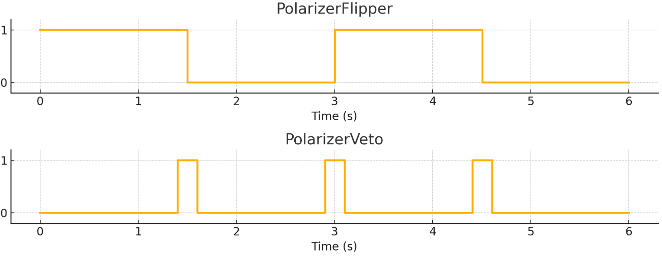
There is a adjustment time period when a flipper changes value during which the state of the flipper is uncertain. Events collected during this time period cannot be assigned to either of the “ON” or “OFF” states, hence they should be discarded in the reduction. The set of time periods for the polarizer flipper are collected in PV PolarizerVeto and for the analyzer flipper in PV AnalyzerVeto.

The image below shows the relation between the flipper and veto logs. Whenever the flipper changes state, there’s a time period during which the veto log becomes 1. During reduction, we’ll use Mantid’s filtering capabilities to discount events collected during these time periods.